
While the basic functions in Excel cover the majority of use cases, there are some situations where a specialized function is more appropriate. In order to find and use specialized functions, you must be familiar with their syntax and understand how they work on a fundamental level.
Topic Objectives
In this topic, you will learn:
- About function categories
- About the Excel function reference
- About function syntax
- About function entry dialog boxes
- Using nested functions
- About automatic workbook calculations
- How to show and hide formulas
- How to enable iterative calculations
Function Categories
Every built-in function that is available in Excel has been categorized into one of 12 standard categories. These categories are available on the Formulas tab, with some categories available under the More Functions drop-down menu:
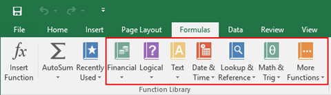
(Note that you can expand the number of standard categories using add-ons.)
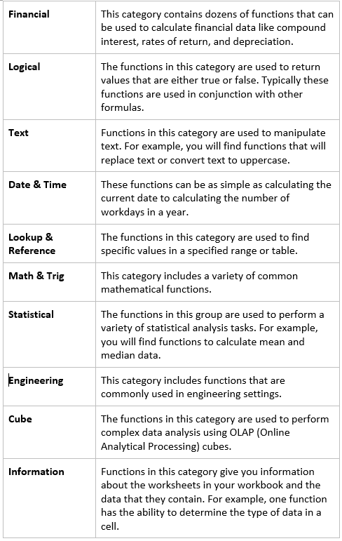
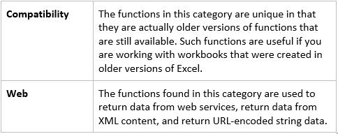
Here is a breakdown of what types of functions each of the available categories contains:
The Excel Function Reference
While you become familiar with many of Excel’s functions, there may be a few that elude you. In such cases you will need to identify which function serves which purpose. This is where the Excel function reference can be invaluable.
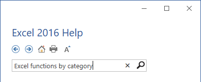
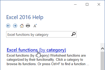
The Excel function reference is a Help resource that will list all of the functions that are available in Excel 2016, what they do, their syntax, and examples of their use. To access the Excel function reference, open the Excel Help window by pressing F1. Next, type “Excel functions by category” into the search field and press Enter:
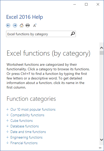
From the list of results, click the “Excel functions (by category)” option:
You will then be able to view all of the functions that Excel 2016 has to offer:
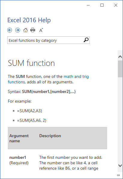
Clicking on any function that is listed here will provide you with much more detail about it:
Instructor Tip: This information is also available at https://support.office.com/en-us/article/Excel-functions-by-category-7fd9655a-4e87-400a-ae5c-c48f16afde0c.
Function Syntax
Functions are a major part of what makes Excel so popular, so now you will explore some different types of functions and learn some tricks that you can use to perform complex calculations. Just keep in mind that even the most complex of formulas can be broken down into simple parts. Remember to pay attention to the order of precedence (using the BEDMAS acronym) and the number of parentheses you use.
The SUMIF Function
=SUMIF(range, criteria, [sum_range])
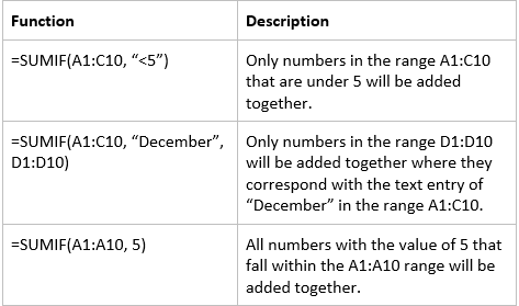
The SUMIF function is used to calculate the sum of values in a specified range if they meet a specified criteria. For example, you could calculate total sales figures and only include numbers that are less than a specified value. The sum_range argument is optional; you can use it if you want to add cells to the sum other than those specified in the argument. If you choose to leave out this argument, the function will only calculate the sum of the values from the previous range argument.
Below are some example of the SUMIF function in action:
The AVERAGEIF Function
=AVERAGEIF(range, criteria, [average_range])
The AVERAGEIF function will return the average of every cell within a range if the specified criteria is met. For example, if you wanted to calculate the average sale amount in a set range of sales data only for sales below a certain amount you could use this function. The average_range argument is optional; it can be used if you want to add cells to the sum other than those specified by the range argument. If you choose to leave out this argument, the function will only calculate the average of the values from the range argument.
Below are some AVERAGEIF functions in action:

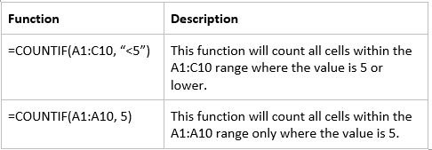
The COUNTIF Function
=COUNTIF(range, criteria)
The COUNTIF function will count the number of cells in a specified range if the criteria is met. For example, this function could be used to count the number of sales associates who have sold X number of products.
IFS Functions
The functions that have been covered so far (AVERAGEIF, COUNTIF, and SUMIF) all have an equivalent IFS function that allow you to perform those respective calculations on data that requires more than just one specified criteria.
With a few exceptions, such functions have very similar syntax:
=SUMIFS(sum_range, criteria_range1, criteria1, [criteria_range2], [criteria2], …)
=AVERAGEIFS(average_range, criteria_range1, criteria1, [criteria_range2], [criteria2], …)
=COUNTIFS(criteria_range, criteria1, [criteria_range2], [criteria2], …)
The COUNTA Function
=COUNTA(value1, [value2],…)
The COUNTA function is used to count the number of cells specified by the argument (value1, value2, etc.) that are not empty.

Function Entry Dialog Boxes
Functions can be entered into a worksheet using a number of different methods. Perhaps the most straightforward is to type the function directly into the Formula Bar – just like a regular formula. For example, if we wanted to use the SUM function to calculate the sum total of the values inside the A1:A6 range, we would select the cell where the result will be displayed and type “=SUM(A1:A6)” into the formula bar:
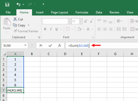
Pressing Enter or clicking the Enter button will then enter the function into your worksheet and then produce the result:
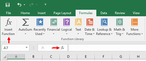
While manually entering a function into the Formula Bar can often be the fastest way to enter a function, it is sometimes a difficult method to take advantage of when you are unsure of a function’s syntax. In such cases, you want to open the Insert Function dialog box. To open this dialog box, first select the cell in which you want the result of the function entered and then click Formulas → Insert Function, or click the Insert Function button that is beside the Formula Bar:
The Insert Function dialog box provides you with a search area (1) that you can use to find a particular function that you need, as well as a category drop-down menu (2) that will display all of the functions that belong to a specified category:
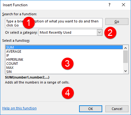
Lower in this dialog box you will see a list of functions (3) that are shown based on your search or the category that you selected. Clicking any of the functions that are listed here will show you a preview (4) of what the syntax for the selected function is and a brief description of what that function is used for.
Once you find and select a function, click OK to enter it into your worksheet. This action will typically display the Function Arguments dialog box:

Using the controls in this dialog box, you are able to add arguments to the function that you selected. For this example, as we are working with the SUM function, we are able to choose data ranges that will be entered into the function for us. You will also see the result of the formula shown near the bottom and the middle of this dialog box.
Clicking the OK button will enter the function into the worksheet using the arguments that you selected.
Using Nested Functions
Some situations require for a function to be nested inside of another function. This means that you are using the results of the nested function as arguments. For example, here is an example of a nested function:
=IF(SUM(A1:A5)>10, SUM(A6:A10), 0)
In this example a two SUM functions have been nested inside of a single IF function. The way this example works is that IF the SUM of data in cells A1:A5 is greater than 10, then this formula will SUM the values of cells A6:A10 and display that result. IF the SUM of data in cells A1:A5 is less than 10, then “0” will be displayed instead.
Automatic Workbook Calculations
By default Excel workbooks with automatically calculate the results of formulas automatically. Occasionally, you may want to switch your workbook calculations to manual recalculation so that you have more control over when formulas are calculated in your workbook. Typically you would do this if you are working with a particularly large workbook and the response times in Excel are slowed when you change a value and numerous formulas calculate the results of this change at the same time.
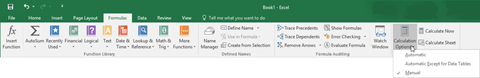
To change the calculation options, click Formulas → Calculate Options. This drop-down command includes the Automatic (default), Automatic Except for Data Tables, and Manual options:
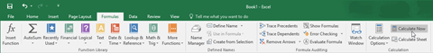
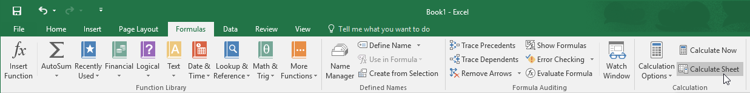
If you switch to the Manual option, you can then calculate formulas in your workbook manually by clicking Formulas → Calculate Now:
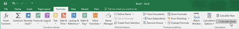
Alternatively, you can also choose to calculate only those formulas on the current worksheet by clicking Formulas → Calculate Sheet:
Showing and Hiding Formulas
To make creating and reviewing worksheets a bit easier, you can show the formulas (instead of the result) on the worksheet and the printed page. To do this, click Formulas → Show Formulas:
Instructor Tip: You can toggle this display with the Ctrl + ` shortcut.
This action will show formulas within the sheet instead of the calculated results:
Enabling Iterative Calculations
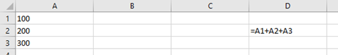
While you would typically want to avoid circular references (formulas that refer to cells that contain the same formula), there are situations where this is desirable. In Excel, you are able to accommodate such situations by enabling iterative calculations and choosing the exact number of iterations required. Iterative calculations are those calculations that repeat until a desired condition is reached. Typically these are used when building more complex calculations, such as those used to calculate tax accrual.
To enable iterative calculations, first open the Excel Options dialog box by clicking File → Options. Next, display the Formulas category. Finally, check the “Enable iterative calculation” check box:
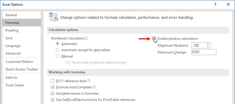
With iterative calculation enabled, any formulas that contain circular references will calculate up to the value found in the Maximum Iterations increment box (100 by default). The Maximum Change text box contains the maximum change value (.001 by default) to control how much the results change.
Activity 1-2
Using Specialized Functions
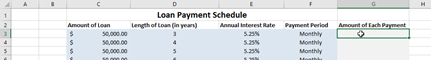
You have a large worksheet that contains the details of dozens of loans. A payment rate for each loan must be calculated according to the terms that have been provided for each. You will use the PMT function to complete this task.
- To begin, open Activity 1-2 from your Exercise Files folder:
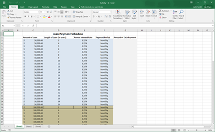
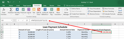
2. First, click to select cell G3:
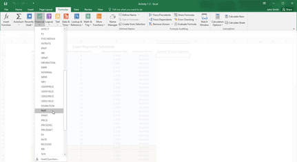
3. Next, click Formulas → Financial → PMT:
4. The Function Arguments dialog will appear. Within this dialog you need to enter all of the arguments. As the interest rate is stored in cell E3, type “E3” into the Rate text box:
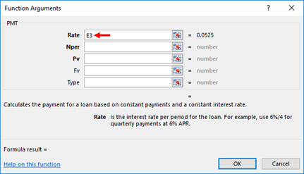
5. As these are annual interest rates and the payments will be monthly, you need to divide this value by 12. Type “/12” following the cell reference in the Rate text box:

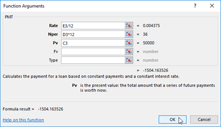
6. The next argument is Nper, or the number of payment periods over the life of the loan. This information is in cell D3, but it is given in years. Because you need to enter it as months, type “D3*12” into the Nper text box:

7. The next argument is Pv, or present value. This is the amount of money that is being borrowed. This information is in cell C3, so type “C3” into the Pv text box:

8. Leave the Fv (Future Value) argument field empty. This argument will default to 0, which is what we want. (This means there will be no part of the loan left outstanding at the end of the payments.) We will also let the Type field default to 0, meaning payments will be due at the end of the payment period. Click OK to create the function:
9. Now you will now have a result in the cell G3. You will also see the PMT function in the Formula Bar:
10. Now it is time to enter this formula for the rest of the data rows. To do this, click cell G3 to make it active, and then drag the AutoFill handle in the lower right corner of the cell down to G94:
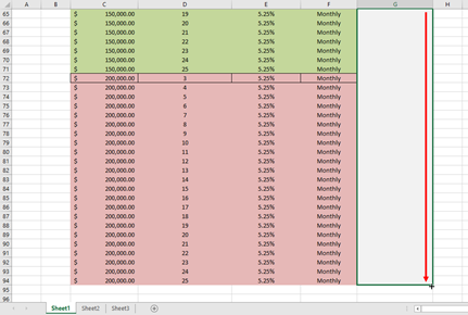
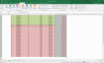
11. Release the mouse button. You will see that the loan payments for each entry have been calculated:
12. Save your work as Activity 1-2 Complete and then close Microsoft Excel 2016.
Summary
Over the course of this lesson you learned about range names and how to apply them. Additionally, you learned about the different function categories and specialized functions that are available. You should also now be familiar with function syntax, nested functions, automatic workbook calculations, and iterative calculations.
Review Questions
- Where do you type in a new range name for a selected range?
You type a new range name for a selected range into the Name Box.
2. How many default function categories are there in Microsoft Excel 2016?
In Excel 2016, there are 12 default function categories.
3. What is the command sequence to show formulas rather than calculated values in cells?
The command sequence to show formulas rather than calculated values in cells is Formulas → Show Formulas.
4. What is a nested function?
A function within the arguments of another function.
5. What is the command sequence to change workbook calculations to manual?
The command sequence to change workbook calculations to manual is Formulas → Calculate Options → Manual.