
To help ensure that everyone who works on the same workbook can understand what formulas and calculations are doing, it is important to use cell and range names. While cell references can be used to identify where formulas are getting information to calculate data, it is not always obvious. Excel allows you to give individual cells and cell ranges names, and then use those names in formulas and functions. Then, you can tell at just a glance what the data is and it is being used.
Topic Objectives
In this topic, you will learn:
- About cell and range names
- How to add range names using the Name box and the New Name dialog box
- How to edit and delete range names
- How cell and range names are used in formulas
Range Names
Range names are meaningful labels that you can assign to
individual cells or cell ranges. You can use a range name anywhere you would use a cell reference or cell range reference. This means you can use a name like “Employees” to describe a range of cells rather than their reference (such as C2:C55).
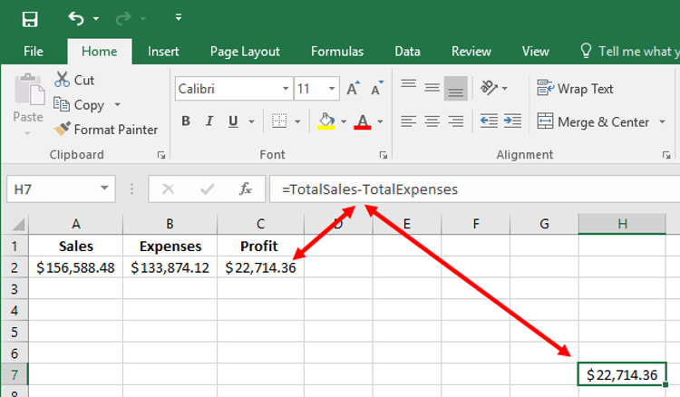
For example, consider the following worksheet. Cells A2 and B2 have been given names (TotalSales and TotalExpenses, respectively) and those names have been used in a formula in cell C2 (=TotalSales-TotalExpenses):

As an added bonus, range names use absolute cell references. This means that if you copy a formula or use AutoFill while using named ranges, the formula will maintain its original cell references:
Range names make formulas much more readable, improve worksheet clarity, and greatly improve worksheet organization. Range names can even help in overall design of your worksheet.
Most small worksheets are usually constructed by filling a sheet with data and then performing calculations. However, range names enable you to create a worksheet by doing the opposite: constructing formulas and then adding the data. When you are designing your worksheet, you can create formulas using names instead of traditional cell references, and then define the names for the corresponding ranges as data becomes available.
For example, below is an empty worksheet with a defined formula but no defined names, which results in a #NAME error. This error will remain visible until both “Value1” and “Value2” have been defined:

Keep in mind when choosing cell or range
names that all names must start with a letter, underscore, or backslash. Beyond
the first character, you can add any letter or number or you wish.
Additionally, names cannot contain any spaces, nor can they contain cell
references. Finally, it is important to know that cell and range names are not case-sensitive.
Adding Range Names Using the Name Box
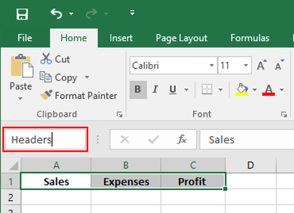
To apply a cell name or range name, first use your cursor to select the cell(s) that you want to name. Next, type the name that you would like to use into the Name Box:
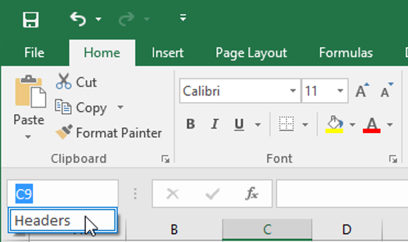
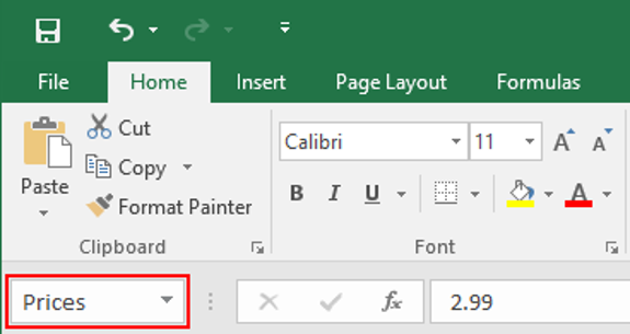
Pressing Enter will apply this name. From then on, you will be able to select this range by clicking the Name Box drop-down menu and clicking on the range name that you set:
Instructor Tip: You can also use the Apply Names dialog box, which is opened by clicking Formulas → Define Name → Apply Names.
Adding Range Names Using the New Name Dialog Box
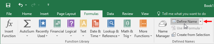
Cells and cell ranges can also be named using the New Name dialog box. While this technique takes a little bit longer, you have more control over what cells the name refers to. To open the New Name dialog box, click Formulas → Define Name:
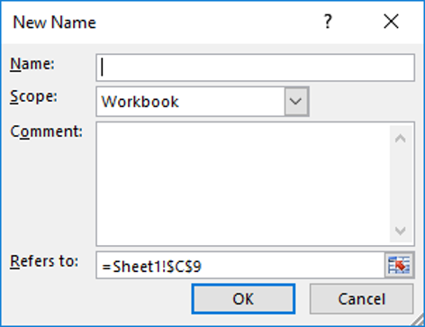
When the New Name dialog box is displayed, you will see that the Name field appears at the top. The Scope drop-down menu allows you to choose if this new name will be applied to only the current worksheet or the entire workbook. Inside the Comment text area you can enter a brief description of the named cell or range. By default, the cells that were selected when the Define Name command was clicked will already be filled into the “Refers to” field. If you wish, you can change this selection by clicking on the cell selector (![]() ):
):

Once you enter your options and click OK,
the named range will be created.
Editing a Range Name and Deleting a Range Name
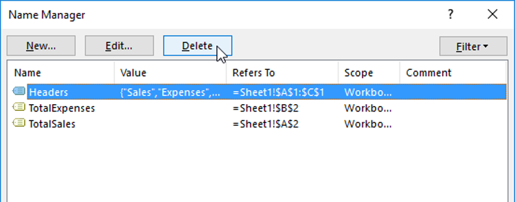
As workbooks are typically dynamic in nature, the ability to manage named cells and ranges can become very important. The Name Manager dialog box allows you to view and manage all named objects within your workbook. This dialog box is accessed by clicking Formulas → Name Manager:
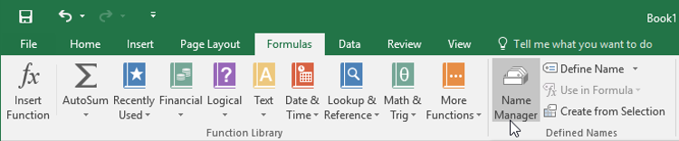
Instructor Tip: You can also use the Ctrl + F3 shortcut.
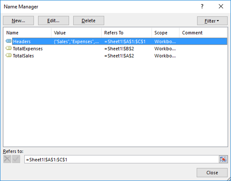
When open, the Name Manager dialog box will list any named objects within the current workbook:
Clicking the New button will open the New Name dialog box, which you can use to create a new range name:
If you select a name from the list in the Name Manager dialog box and then click the Edit button, the Edit Name dialog box will be shown:
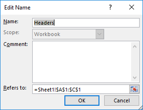
This dialog box is identical to the New
Name dialog box; the only difference is that it will be prepopulated with information
from the selected range name.
To delete a range name, click to select the range name in question and then click the Delete button:
A dialog will then open to ask you to confirm this action. Click OK to complete the deletion process.
Finally, the Filter command is used to show only certain ranges based on specified criteria:

This is particularly useful when working with a workbook that contains a large amount of range names, as you can quickly narrow down the list to only those ranges that you would like to work with.
Using Range Names in Formulas
Cell and range names are not just useful in
keeping your workbooks more organized; they can also help immensely in the
creation of formulas. This is because after you have defined a cell or range
name, you are able to use that name in place of the usual cell reference. This makes
formulas much more readable.
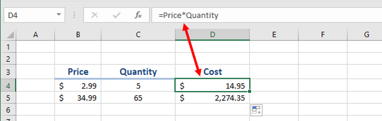
For example, below you can clearly and quickly see what this formula does. If it used standard cell references, it would be much harder to tell:
Perhaps one of the easiest methods to enter cell and range names into a formula is to use the Formula AutoComplete feature. Just like how the AutoComplete feature suggests function names based on the first few characters that you type into the Formula Bar, it will also suggest cell and range names in a small menu. Double-clicking on a suggestion in this menu will insert it into the formula:
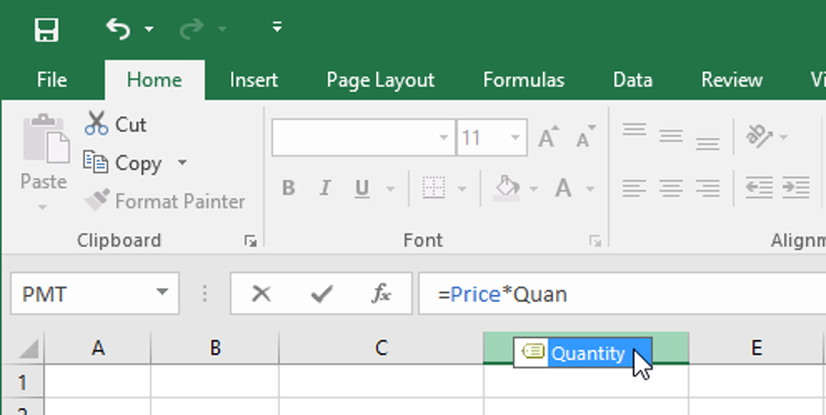
You can differentiate names from functions and other objects suggested by the small tag icon that appears by each name ( ![]() ).
).
In addition to manually entering cell and range names, you can also use the Use in Formula command to insert existing cell and range names into formulas. To access this command, click Formulas → Use in Formula:
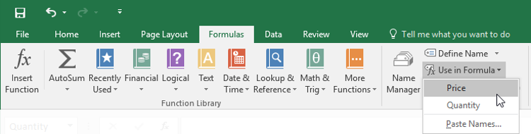
This action will display a drop-down menu listing all of the existing cell and range names. Clicking on an option will insert its reference into the Formula Bar.
Activity 1-1
Using Range Names in Formulas
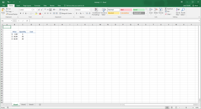
Using the features that you learned about in this topic, you will complete a small sales worksheet that you have been working on.
- To begin, open Activity 1-1 from your Exercise Files folder:
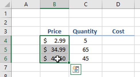
2. To create the first range name, use your cursor to select cells B4:B6:
3. Next, type “Prices” inside the Name Box. Press Enter:
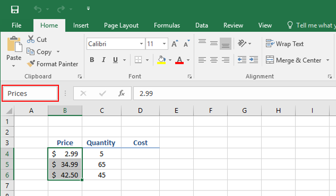
4. The selected range will now have “Prices” as a range name:
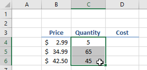
5. Now, let’s try another method to create another range name. First, use your cursor to select cells C4:C6:
6. Next, click Formulas → Define Name:

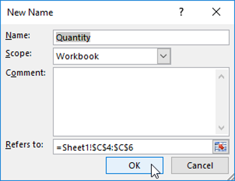
7. The New Name dialog box will now be displayed. Ensure that “Quantity” appears inside the Name text box and that the Scope drop-down menu is set to Workbook. Click OK:
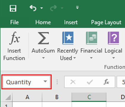
8. The selected range now has “Quantity” as a range name:
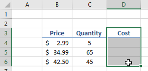
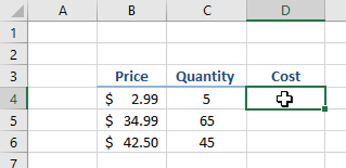
9. You have one more range name to create. Use your cursor to select cells D3:D6:
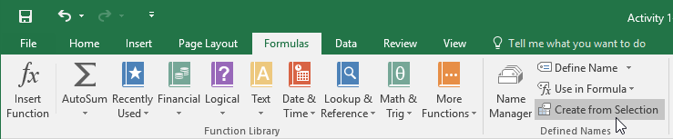
10. Click Formulas → Create from Selection:
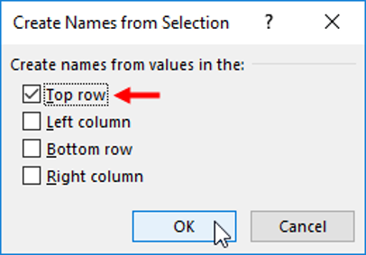
11. In the Create Names from Selection dialog box, ensure that the “Top row” checkbox is selected and click OK:
12. Next, you need to create a formula that will calculate the cost of the items (Quantity*Price). Select cell D4:
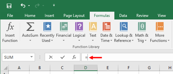
13. Click inside the Formula Bar and type “=”:
14. Next, type “Prices” followed by an asterisk:

Note that because Prices is a range name, its text will appear blue in the Formula Bar and blue shading will appear around that range of data on the worksheet.
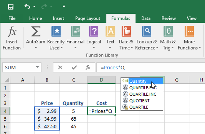
15. Still inside the Formula Bar, type “Q” and then double-click the Quantity result from the small menu that appears:
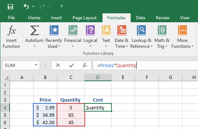
16. The Quantity name will now appear within the Formula Bar in red text, with its associated range shaded in red in the worksheet:
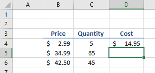
17. Press Enter to apply the formula. You will see the result appear in D4:
18. Save the current workbook as Activity 1-1 Complete and then close Microsoft Excel 2016.